


Most fleet spare parts reorder point lead time variability calculators give you clean formulas that work great until your primary supplier's warehouse floods and suddenly those 3-day filters become 45-day backorders. That's when you realize your inventory math missed something fundamental.
Running parts inventory for a 200-vehicle fleet isn't like managing retail stock. When a transmission filter runs out and you've got three buses waiting, you're looking at $4,800 daily in lost revenue plus angry customers. The math matters differently when downtime compounds across interconnected systems.
The real cost structure behind parts criticality
Parts criticality isn't about whether something's expensive. A $12 cabin air filter and a $1,200 ECM module might seem obviously different in priority, but that filter keeping driver comfort systems running prevents $340 daily in driver overtime from heat-related slowdowns during summer routes.
Tier 1 - Revenue stoppers - These parts directly halt vehicle operation. No brake chambers means no bus moves. No fuel pump means no delivery happens. Vehicle down equals revenue gone.
Tier 2 - Cascade failures - Parts that trigger multiple issues when unavailable. A failed HVAC compressor clutch might seem minor until drivers start refusing routes in 95-degree weather, triggering union grievances and forcing expensive rental substitutions.
Tier 3 - Efficiency degraders - Components affecting operational tempo but not stopping it. Worn suspension bushings mean slower speeds, more fuel burn, driver fatigue. The cost accumulates through decreased productivity rather than hard stops.
Tier 4 - Compliance maintainers - DOT inspection items that don't affect immediate operation but trigger fines and out-of-service orders. Marker lights, mudflaps, reflective tape. The cost hits through regulatory action, not operational failure.
Safety stock mathematics with real lead-time chaos
Standard safety stock formulas assume lead times follow nice distributions. Reality looks different when your supplier network includes regional distributors, OEM warehouses, and aftermarket vendors with wildly different reliability patterns.
Prevent costly breakdowns with proactive maintenance.
Fleetelyly helps you schedule, track, and manage every vehicle service efficiently.
- Automated maintenance reminders
- Real-time service tracking
- Parts inventory integration
No credit card required
Take oil filters for a mixed fleet. Your primary supplier delivers in 3-5 days normally. But during peak season, those same filters jump to 12-15 days. Your backup supplier maintains 7-day consistency but costs 40% more. The third option ships from overseas with 30-45 day variability but 60% lower cost.
The working formula adjusted for this reality: Safety Stock = Z-score × √(Lead Time × Demand Variance² + Average Demand² × Lead Time Variance²)
Making this practical with actual numbers: You're managing filters for 85 diesel vehicles. Daily consumption averages 3.2 filters with standard deviation of 1.8. Primary supplier lead time: 4 days average, 2.3 days standard deviation. Target service level: 95% (Z-score = 1.65).
Safety Stock = 1.65 × √(4 × 1.8² + 3.2² × 2.3²) Safety Stock = 1.65 × √(12.96 + 54.17) Safety Stock = 1.65 × 8.2 Safety Stock = 14 filters (rounded up)
The formula misses this: your primary supplier has a 15% chance of complete stockout lasting 10+ days based on last year's data. The real safety stock needs a second calculation layer.
Decision tables that match operational reality
Min/max levels need different logic for different part categories. Working decision matrix based on actual fleet patterns:
| Part Category | Lead Time Variance | Daily Usage | Min Stock Formula | Max Stock Formula |
|---|---|---|---|---|
| Tier 1 High-Turn | <30% | >2 units | SS + (LT × DU × 1.5) | Min × 2.5 |
| Tier 1 Low-Turn | >30% | <0.5 units | SS + (Max LT × DU) | Min × 3 |
| Tier 2 Predictable | <20% | Any | SS + (LT × DU) | Min × 2 |
| Tier 2 Variable | >50% | Any | SS × 1.5 + (Max LT × DU) | Min × 2.5 |
| Tier 3/4 Standard | Any | >1 unit | (LT × DU × 1.2) | Min × 1.8 |
| Tier 3/4 Sporadic | Any | <0.2 units | Fixed 2 units | Fixed 5 units |
The formulas adapt based on consumption patterns. High-turnover tier 1 parts get aggressive minimums because stockouts hurt immediately. Low-turnover critical parts get even higher buffers because usage spikes unpredictably when multiple vehicles need service simultaneously.
These numbers come from tracking actual fleet behaviors. When buses cluster their maintenance schedules, you might burn through 15 air filters in one day instead of the usual 3.
Worked example: Brake chamber inventory optimization
Setting reorder points for brake chambers on a 120-vehicle transit fleet with mixed bus types.
Current situation:
-
Fleet uses Type 30 chambers across all vehicles
-
Average weekly consumption
8 chambers
-
Usage pattern
clustered (multiple chambers often fail together)
-
Primary supplier lead time
5-7 business days
-
Secondary supplier
14-21 days at 30% lower cost
-
Emergency supplier
Next-day at 280% cost
Step 1: Calculate base demand during lead time Primary supplier average: 6 days, Daily usage: 8/5 = 1.6 chambers, Base demand: 6 × 1.6 = 9.6 chambers
Step 2: Assess lead time variability impact Lead time standard deviation: 1.4 days, Demand standard deviation: 2.3 chambers per week = 0.46 daily, Combined variability = √(6 × 0.46² + 1.6² × 1.4²) = √(1.27 + 5.02) = 2.51
Step 3: Set safety stock for 97% service level Z-score for 97% = 1.88, Safety stock = 1.88 × 2.51 = 5 chambers (rounded)
Step 4: Determine reorder point Reorder point = Base demand + Safety stock = 10 + 5 = 15 chambers
Step 5: Set min/max levels considering clustering Since chambers fail in clusters (usually 2-4 at once):
-
Minimum stock
15 chambers (reorder point)
-
Maximum stock
15 × 2.2 = 33 chambers
This accounts for the reality that when one chamber fails, mechanics often find 2-3 more marginal ones during inspection.
Handling multi-supplier complexity
Fleet operations juggle 3-5 suppliers per part category based on availability, price breaks, and payment terms. The textbook approach suggests choosing one supplier and optimizing around their lead times.
For high-criticality parts, the strategy looks like: Primary supplier handles 70% of regular flow at standard pricing with predictable lead times. You maintain blanket POs here with scheduled releases. Secondary supplier provides 20% during primary stockouts or price spikes. Their higher lead time variance gets offset by maintaining separate safety stock calculations. Emergency supplier covers the remaining 10% for crisis situations. Yes, you're paying 3x normal price, but that's cheaper than deadline penalties or stranded vehicles.
Keep a reserved emergency allocation for Tier 1 parts to reduce repeated expensive emergency orders.
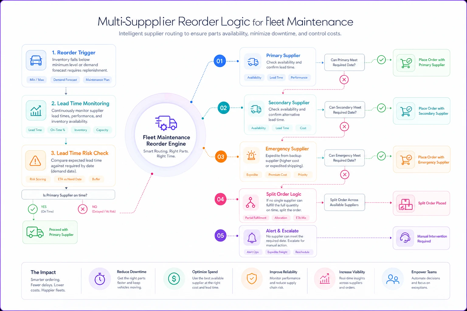
The reorder logic adjusts dynamically. When primary inventory drops below reorder point, order from primary. If primary lead time exceeds 150% normal, split order between primary and secondary. If combined lead time threatens stockout, trigger emergency supplier for bridge inventory.
This gets complex fast. Most spreadsheets break down when you're tracking 8-10 different scenarios for every part.
Creating actionable reorder triggers
Static reorder points fail when demand patterns shift seasonally or equipment ages. Your brake pad consumption in January looks nothing like July, and five-year-old vehicles burn through components faster than new additions.
Consumption velocity triggers - Track 7-day rolling average consumption. When it exceeds historical average by 40%, temporarily boost reorder points by the same percentage. This catches wear pattern changes before stockouts hit.
Lead time deviation triggers - Monitor supplier performance weekly. When average lead time increases 25% over trailing 30 days, automatically increase safety stock by: Additional SS = Z-score × Average Demand × (New LT - Old LT)
Criticality escalation triggers - Parts moving from Tier 3 to Tier 2 criticality (maybe new regulations made them inspection items) get automatic reorder point adjustments. The calculation shifts from efficiency-based to availability-based formulas.
These triggers prevent the common problem where reorder points stay static while operating conditions change. Most fleets update their calculations quarterly or annually. By then, you've already had the stockouts.
Technology integration without complexity
Spreadsheet-based reorder calculations work until you're managing 3,000 SKUs across multiple locations. The formulas become unwieldy, updates lag, and someone inevitably breaks the VLOOKUP that feeds everything.
Modern fleet operations benefit from AI-powered operational software that handles the mathematical heavy lifting while maintaining visibility. These platforms track consumption patterns, monitor supplier performance, and adjust reorder parameters automatically based on real usage data rather than theoretical models.
Software handles the routine calculations and pattern detection while managers focus on supplier relationships, contract negotiations, and strategic inventory decisions. When lead times spike or consumption patterns shift, the system flags the change immediately rather than waiting for monthly reviews.
Good inventory management software also centralizes information from multiple sources - maintenance schedules, supplier catalogs, historical consumption, and budget constraints - into unified dashboards. This eliminates the common problem where purchasing doesn't know maintenance just scheduled 20 brake jobs for next week.
You still need to understand what the software is doing and why it's recommending certain stock levels.
Common pitfalls in variable lead time planning
Averaging averages means calculating average lead time across all suppliers creates meaningless numbers. A 7-day average between a 3-day and 30-day supplier doesn't reflect either reality. Track each supplier's performance separately.
Ignoring correlation happens when your alternator supplier has delays, your battery supplier probably does too since they share distribution networks. Safety stock calculations assuming independent failures underestimate risk.
Over-trusting supplier promises - that "guaranteed 5-day delivery" comes with fine print. Track actual performance, not contractual promises. Build safety stock on reality, not sales presentations.
Neglecting shelf life is common with rubber components, fluids, and filters that degrade over time. Maximum stock calculations need expiration constraints. That great bulk deal on coolant hoses becomes expensive waste after 18 months in desert storage.
Assuming normal distributions fails because parts consumption rarely follows bell curves. You get clusters, seasonality, and equipment aging effects. The mathematical models need adjustment for these patterns.
Making the numbers work in practice
Complete worked example for setting up DEF (Diesel Exhaust Fluid) inventory policy for a 95-vehicle fleet:
Fleet profile:
-
60 heavy-duty trucks (2.5 gallons DEF per 100 miles)
-
35 medium-duty vehicles (1.8 gallons per 100 miles)
-
Average daily mileage
180 miles per heavy, 210 miles per medium
-
DEF criticality
Tier 1 (vehicles won't run without it)
Daily consumption calculation:
Heavy trucks: 60 × (180/100) × 2.5 = 270 gallons, Medium vehicles: 35 × (210/100) × 1.8 = 132 gallons, Total daily: 402 gallons
Supplier analysis:
-
Bulk delivery (2,500 gallon minimum)
3-5 day lead time, $2.10/gallon
-
Tote delivery (275 gallons)
Next-day available, $3.40/gallon
-
Emergency drums (55 gallon)
Same-day, $5.80/gallon
Lead time variability assessment:
Bulk delivery standard deviation: 1.2 days. Historical stockout frequency: 2 events in past year lasting 7-10 days each
Safety stock calculation with stockout risk:
Base safety stock (95% service, 4-day average lead): SS = 1.65 × √(4 × 82² + 402² × 1.2²) = 495 gallons Stockout adjustment: Risk-adjusted SS = 495 + (402 × 3) = 1,701 gallons (Adding 3 days coverage for potential stockout)
Reorder point:
RP = (402 × 4) + 1,701 = 3,309 gallons
Min/Max levels:
Minimum: 3,309 gallons (triggers reorder), Maximum: 6,000 gallons (tank capacity constraint)
Operational policy:
-
Primary strategy
Order 2,500 gallons when inventory hits 3,309
-
Backup trigger
If bulk unavailable, order 10 totes (2,750 gallons)
-
Emergency protocol
Deploy drums to sites if below 400 gallons
This policy maintains service levels while managing three different supply channels with vastly different economics and lead times.
The difference between theory and fleet reality
Textbook inventory management assumes stable demand, reliable suppliers, and infinite storage. Fleet operations deal with seasonal swings, supplier bankruptcies, and shop spaces where every square foot counts.
The math provides a framework, but operational judgment determines success. When your model says hold 50 air filters but your senior mechanic says "we'll need 80 for summer PM season," listen to the mechanic. The formula doesn't know your municipality just approved overtime for weekend maintenance blitzes.
When lead time variance calculations suggest huge safety stocks, sanity-check against cash flow reality. Sometimes accepting occasional emergency purchases beats tying up $30,000 in slow-moving inventory.
The goal isn't mathematical perfection but operational resilience. Your reorder policy should keep vehicles running, mechanics working, and costs controlled - in that order. Everything else is optimization around those core requirements.
Building robust inventory policies means embracing the messiness of actual operations while using mathematical frameworks to guide decisions. The formulas matter, but they're tools, not rules. Your fleet's specific patterns, constraints, and risks determine how to apply them.
When software handles the routine calculations and pattern monitoring, managers can focus on what matters: maintaining relationships with suppliers, identifying emerging risks, and ensuring the parts room supports the shop floor. That combination of mathematical rigor and operational wisdom keeps fleets running regardless of how variable those lead times become.
Ready to maximize fleet uptime and reduce maintenance costs?
Join 2,000+ fleet managers using Fleetelyly to streamline maintenance workflows and improve vehicle reliability.